Introductory: Nitrogen#
In this introductory tutorial, we will explore how to
create a molecular structure,
perform a geometry optimization,
obtain the Hessian
in the ASE framework, and finally how to start a JEDI analysis and interpret its results.
We will use nitrogen as a minimal system with only two atoms and one bond, as it contains all essential ingredients for a strain analysis. EMT is used for convenience because it is fast, readily available in ASE, and sufficient to illustrate the workflow, even though it is not necessarily quantitative.
Complete Example#
Here, you find the whole code example to test. Below, every step is discussed in detail.
from ase import Atoms
from ase.calculators.emt import EMT
from ase.optimize import BFGS
from ase.vibrations import Vibrations
from strainjedi.jedi import Jedi

# Create a structure
atoms = Atoms('N2', [(0, 0, 0), (0, 0, 1.1)])

# Set up calculator
atoms.calc = EMT()

# Optimize geometry
BFGS(atoms).run(fmax=0.01)

# Calculate vibrational modes (Hessian)
vib = Vibrations(atoms)
vib.run()
modes = vib.get_vibrations()

# Create a distorted structure based on the optimised geometry
atoms_distorted = atoms.copy()
atoms_distorted.positions[1][2] += 0.1

atoms_distorted.calc = EMT()
atoms_distorted.get_potential_energy()

# Run JEDI analysis
jedi = Jedi(atoms, atoms_distorted, modes)
jedi.run()

# Open visualisation window
jedi.visualize(show=True, single_mode='bl')
Creating the Structure#
First, we will need a structure to analyse: as discussed, we choose a nitrogen molecule for that.
The Atoms object from ASE aids us in defining the structure: Two nitrogen atoms, and a reasonable starting distance between the atoms for the later conducted optimization.
from ase import Atoms

atoms = Atoms('N2', [(0, 0, 0), (0, 0, 1.1)])  # 1.1 Angstrom
Selecting a Calculator#
JEDI itself does not perform geometry optimizations and instead relies on established calculators to do the “hard work” up front. Here, we attach an EMT calculator to the structure.
from ase.calculators.emt import EMT

atoms.calc = EMT()
Optimizing the Geometry#
Just attaching a calculator doesn’t do much by itself for our purposes, but it enables us to ask for an optimization.
In this case, we use the BFGS algorithm as implemented by ASE.
Further, by setting fmax=0.01, we ask ASE to optimize the structure quite well by restricting the maximum allowable force on all individual atoms.
from ase.optimize import BFGS

BFGS(atoms).run(fmax=0.01)
Calculating the Hessian#
Now that we performed a geometry optimization by means of BFGS, we can obtain the Hessian of the relaxed structure as a VibrationsData object.
from ase.vibrations import Vibrations

vib = Vibrations(atoms)
vib.run()
modes = vib.get_vibrations()
Creating a Strained Structure#
JEDI operates on a pair of geometries: a relaxed reference structure and a strained configuration. The strained structure can originate from MD snapshots, constrained optimizations, or experimental geometries. Here, we simply introduce a small Cartesian displacement to generate a test strain field.
atoms_distorted = atoms.copy()
atoms_distorted.positions[1][2] += 0.1
Evaluating the Strained Structure Energy#
The energy of the strained structure is required for the comparison between the harmonic strain estimate and the corresponding electronic energy difference. This value is used internally when assessing the quality of the harmonic approximation.
atoms_distorted.set_calculator(EMT())
atoms_distorted.get_potential_energy()
Running the JEDI Analysis#
JEDI takes three inputs:
equilibrium geometry and energy as an
Atomsobject,strained geometry and energy as an
Atomsobject,Hessian of the equilibrium geometry as a
VibrationsDataobject.
From these, it performs the coordinate transformation of the Hessian, evaluates the strain distribution in internal coordinates, and computes the harmonic strain energy.
from strainjedi.jedi import Jedi

jedi = Jedi(atoms, atoms_distorted, modes)
jedi.run()
Results#
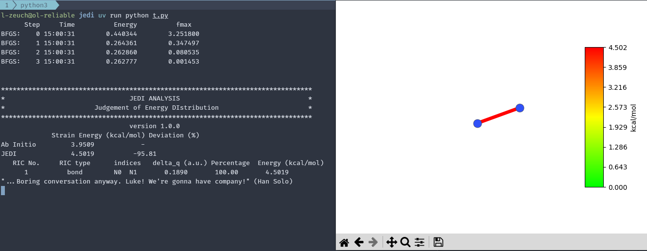
Running the discussed code should yield a printout to your console similar to the one below.
      Step     Time          Energy          fmax
BFGS:    0 11:31:04        0.440344        3.251800
BFGS:    1 11:31:04        0.264361        0.347497
BFGS:    2 11:31:04        0.262860        0.080535
BFGS:    3 11:31:04        0.262777        0.001453


************************************************************************************************************************
*                                                    JEDI ANALYSIS                                                     *
*                                           Judgement of Energy DIstribution                                           *
************************************************************************************************************************
                                                     version 1.1.0
                    Strain Energy (kcal/mol)     Deviation (%)
Ab Initio                    3.9509                    -
JEDI                         4.5019                  13.95
      RIC No.             RIC type            indices          delta_q (a.u.)        Percentage      Energy (kcal/mol)
         1                  bond               N0  N1              0.1890              100.00              4.5019
For this system, strain is confined to the N–N stretching coordinate due to the absence of additional internal degrees of freedom. Key outputs are the strain energy and its decomposition in internal coordinates, along with the comparison between harmonic and ab initio energy differences (from electronic structure calculations). This deviation is a measure for the applicability of the harmonic approximation to the deformation experiment.
Visualisation#
While terminal/text output is useful for storing and later analysis, it is decidedly hard to interpret; for that reason, we provide a simple way to visualize the results via Matplotlib. Add the following line to the end of the above code and re-run the script.
jedi.visualise(show=True, single_mode='bl')
This will launch a Matplotlib window visualizing the strain distribution in the molecule after the analysis is finished.
Setting single_mode to 'bl' ensures that only the energy distribution across bonds is considered, since the molecule contains no angles or dihedral angles.