Further Analysis
Due to the larger outputs of the following examples, the outputs are attached as files and only the visualizations are shown. The calculations were performed with low accuracy to keep the computational effort as low as possible so that the first time user can perform them to getting used to Jedi. Nevertheless, the Vasp calculations might still take very long. For better results, a higher accuracy is needed. Note that the usage of the gaussian and vasp calculators still needs the respective licences. If you do not have a licence you can use other programs like ORCA or GPAW.
Custom bonds
Custom bonds can be analyzed too. The Jedi package has a function to determine hydrogen bonds in a structure. These will be added to the RIC with add_custom_bonds() after generating the Jedi object.
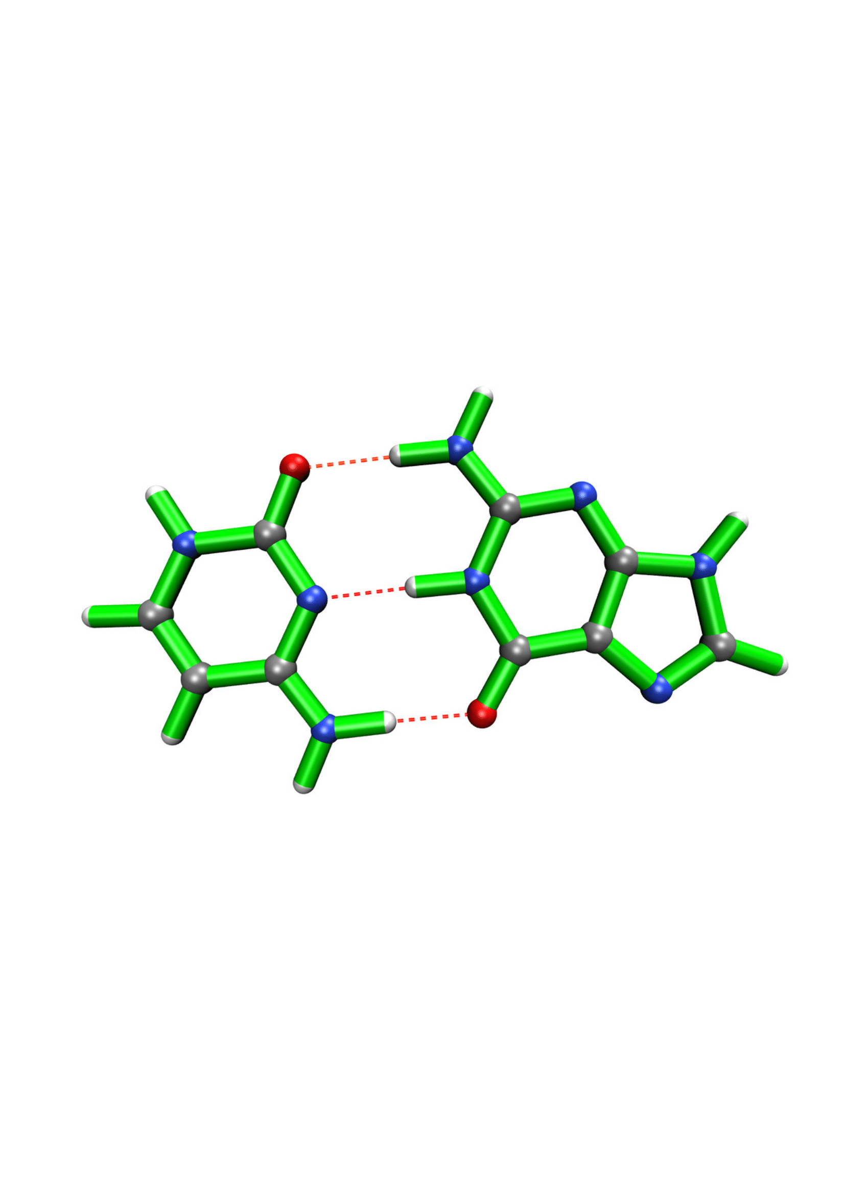
Stretching Hydrogen Bonds Using COGEF
Here, cytosine and guanine are examined.
from strainjedi.io.gaussian import Gaussian, GaussianOptimizer, get_vibrations
import ase.io
from strainjedi.jedi import Jedi, get_hbonds
from ase.vibrations.vibrations import VibrationsData

mol = ase.io.read('cg.xyz')

calc = Gaussian(mem='6GB',
                    label='opt',
                    method='blyp',
                    basis='4-21G',
                    EmpiricalDispersion='GD3BJ',
                    scf='qc')
opt=GaussianOptimizer(mol,calc)
opt.run(fmax='tight', steps=100)
ase.io.write('opt.json',mol)

mol=ase.io.read('opt.json')
mol.calc = Gaussian(mem='6GB',
                    iop='7/33=1',
                    freq='',
                    label='freq',
                    chk='freq.chk',
                    save=None,
                    method='blyp',
                    basis='4-21G',
                    EmpiricalDispersion='GD3BJ',
                    scf='qc')
mol.get_potential_energy()
hessian = get_vibrations('freq',mol)
hessian.write('modes.json')

mol2 = mol.copy()
v = mol.get_distance(10,27)+0.1
w = mol.get_distance(13,21)+0.1
x = mol.get_distance(15,20)+0.1

calc = Gaussian(mem='6GB',

                    label='dist',


                    method='blyp',
                    basis='4-21G',
                    EmpiricalDispersion='GD3BJ',
                    scf='qc',addsec='''11 28 ={} B
14 22 ={} B
16 21 ={} B
11 28 F
14 22 F
16 21 F'''.format(v,w,x))
opt=GaussianOptimizer(mol2,calc)
opt.run(fmax='tight', steps=100,opt='ModRedundant')

j = Jedi(mol,mol2,hessian)
j.add_custom_bonds(get_hbonds(mol2))
j.run()
j.vmd_gen()
The input written by ASE for the COGEF calculation has a line break too much between the coordinates section and the constraints section. So it has to be corrected manually and the job needs to be sent manually. The gaussian outputs can be read by the funtions delivered with the Jedi package.
from ase.vibrations.vibrations import VibrationsData
from strainjedi.jedi import Jedi, get_hbonds
from strainjedi.io.gaussian import get_vibrations, read_gaussian_out

file=open('output/opt.log')
mol=read_gaussian_out(file)
file2=open('output/dist.log')
mol2=read_gaussian_out(file2)
modes=get_vibrations('output/freq',mol)
j=Jedi(mol,mol2,modes)
j.add_custom_bonds(get_hbonds(mol2))

j.run()
j.vmd_gen()
Other types of interactions that can be localized between two atoms can added on the same way by giving a 2D array to the add_custom_bonds function.
Analysis of a Substructure
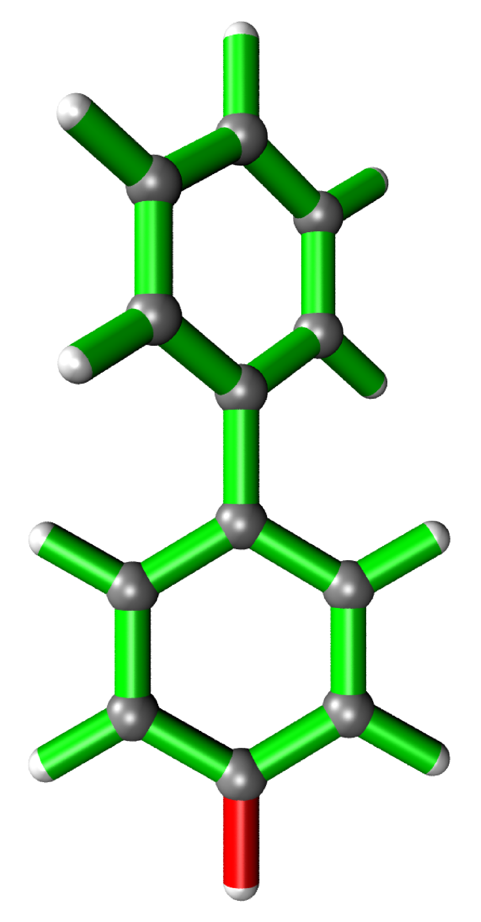
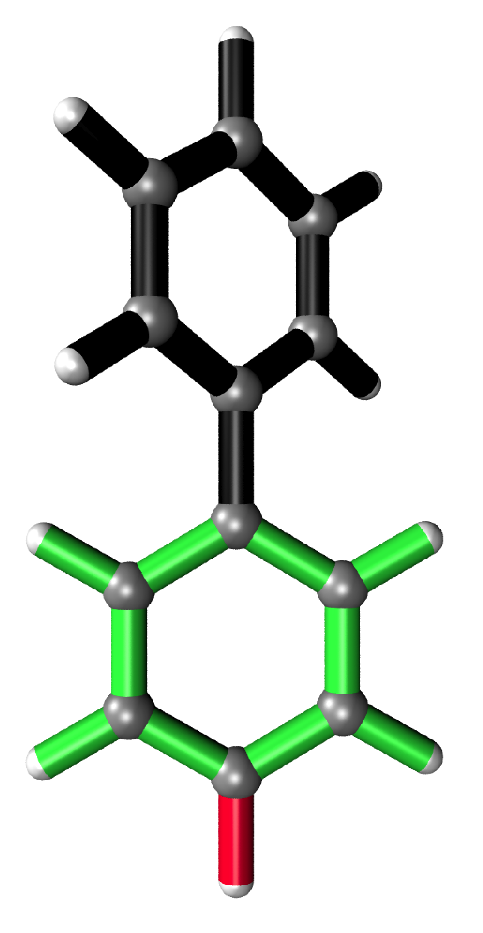
Biphenyl
It is possible to analyse substructures. This is desired when local changes of large structures need to be analysed. Here, a Hydrogen atom in a biphenyl molecule is pulled 0.1 Å away from its relaxed position. For the partial analysis, the hessian of only one phenyl ring is calculated yielding near identical values as when calculated for the whole system.
import ase.io
from ase.calculators.vasp import Vasp
from ase.vibrations.vibrations import VibrationsData
from strainjedi.jedi import Jedi
import os

mol=ase.io.read('start.xyz')

#optimize the molecule
label="opt"
mol.calc=Vasp(label='%s/%s'%(label,label),
                prec='Accurate',
                xc='PBE',pp='PBE',
                nsw=0,ivdw=12,
                lreal=False,ibrion=2,
                isym=0,symprec=1.0e-5,
                encut=315,ediff=0.00001,isif=2,
                command= "your command to start vasp jobs")

mol.calc.write_input(mol)
mol=ase.io.read('opt/vasprun.xml')  #vasp needs a specific ordering of the atoms writing and rereading will adapt this indexing
mol.get_potential_energy()

#frequency analysis
label="freq"
mol.calc=Vasp(label='%s/%s'%(label,label),
                prec='Accurate',
                xc='PBE',pp='PBE',
                nsw=0,ivdw=12,
                lreal=False,ibrion=5,
                isym=0,symprec=1.0e-5,
                encut=315,ediff=0.00001,isif=2,
                command= "your command to start vasp jobs")
mol.get_potential_energy()
hessian=mol.calc.get_vibrations()

c = FixAtoms(indices=[6,7,8,9,10,11,17,18,19,20,21])
mol.set_constraint(c)

label='pfreq'
calc3 = Vasp(label='pfreq/%s'%(label),prec='Accurate', ibrion=5,ediff=0.00001,
            xc='PBE',pp='PBE',ivdw=12,symprec=1.0e-5,encut=315,isym=0,
            lreal=False,command= "sh /home1/wang/vasp/submit-vasp-job.sh -la %s"%(label))

mol.calc=calc3
mol.get_potential_energy()
parthessian=mol.calc.get_vibrations()
np.savetxt('p-hessian',parthessian._hessian2d,fmt='%25s') #VibrationsData.write does not allow saving partial hessian

mol.set_constraint()
#distort molecule
mol2=mol.copy()
v=mol2.get_distance(3,14,vector=True)
v/=np.linalg.norm(v)
positions=mol2.get_positions()
positions[14]+=v*0.1
label='para-C-H'
mol2.set_positions(positions)
calc = Vasp(label='%s/%s'%(label,label),
            prec='Accurate',
            xc='PBE',pp='PBE',
            nsw=0,ivdw=12,
            lreal=False,ibrion=2,
            isym=0,symprec=1.0e-5,
            encut=315,ediff=0.00001,isif=2,
            command= "your command to start vasp jobs")
mol2.calc=calc
mol2.get_potential_energy()

os.mkdir('all')
os.chdir('all')
j=Jedi(mol,mol2,hessian)
j.run()
j.vmd_gen()

os.chdir('../..')
os.mkdir('partial')
os.chdir('partial')
jpart=Jedi(mol,mol2,parthessian)
jpart.partial_analysis(indices=[0,1,2,3,4,5,12,13,14,15,16])
jpart.vmd_gen()

Analysis output
Analysis output
It is possible to only show specific RIC after calculating the whole analysis by giving a list of the desired atoms’ indices to the run function.
os.chdir('../..')
os.mkdir('special')
os.chdir('special')
jpart=Jedi(mol,mol2,modes)
jpart.run(indices=[0,1,2,3,4,5,12,13,14,15,16])
jpart.vmd_gen()

More Examples
The following is intended to be an inspiration of what can also be analyzed.
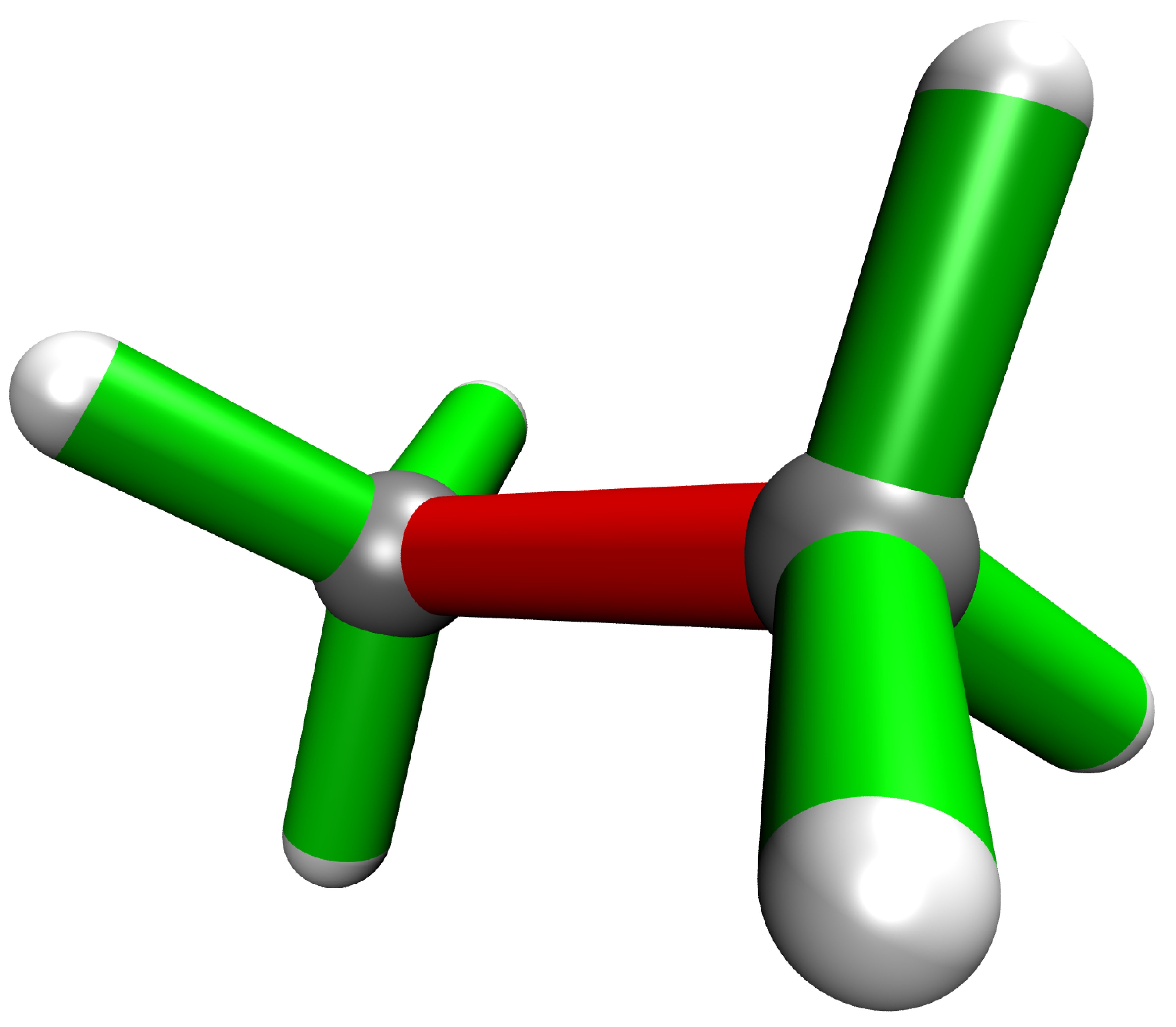
Using EFEI
Stretching bonds using a predefined force is possible with the EFEI method. The following example shows an ethane molecule of which the C-C bond is stretched with a force of 4 nN.
from ase.build import molecule
from ase.vibrations.vibrations import VibrationsData
from strainjedi.jedi import Jedi
from strainjedi.io.orca import OrcaOptimizer, get_vibrations, ORCA
import ase.io

mol=molecule('C2H6')

calc = ORCA(label='opt',
            orcasimpleinput='pbe cc-pVDZ OPT'
            ,task='opt')
opt=OrcaOptimizer(mol,calc)
opt.run()

ase.io.write('opt.json',mol)
mol=ase.io.read('opt.json')
mol.calc=ORCA(label='orcafreq',
            orcasimpleinput='pbe cc-pVDZ FREQ',
            task='sp')
mol.get_potential_energy()

hessian=get_vibrations('orcafreq',mol)

mol2=mol.copy()
calc = ORCA(label='stretch',
            orcasimpleinput='pbe cc-pVDZ  OPT',
            orcablocks='''%geom
    POTENTIALS
        { C 0 1 4.0 }
    end
end ''',task='opt')
opt=OrcaOptimizer(mol2,calc)
opt.run()
ase.io.write('force.json',mol)

j=Jedi(mol,mol2,hessian)
j.run()
j.vmd_gen()
Hydrostatic Pressure using X-HCFF
A lot of models have been developed to simulate pressure. X-HCFF is one of them that simulates Hydrostatic pressure. Here, Dewar and Ladenburg benzene are analyzed under 50 GPa of pressure.
import ase.io
from ase.vibrations.data import VibrationsData
from strainjedi.jedi import Jedi
from strainjedi.io.qchem import get_vibrations, QChemOptimizer, QChem

mol = ase.io.read('Dewar.xyz')

label='opt'

calc=QChem(jobtype='sp',
            label='xhcff/50GB/%s'%(label),
            method='pbe',dft_d='D3_BJ',
            basis='cc-pvdz',GEOM_OPT_MAX_CYCLES='150',
            USE_LIBQINTS='1',MAX_SCF_CYCLES='150',
            command='your command')
mol.calc = calc
opt = QChemOptimizer(mol)
opt.run()


label='freq'
calc=QChem(jobtype='freq',
            label='xhcff/50GB/%s'%(label),
            method='pbe',dft_d='D3_BJ',
            basis='cc-pvdz',vibman_print= '7',
            command='your command')
mol.calc = calc
mol.calc.calculate(properties=['hessian'],atoms=mol)

hessian=get_vibrations(label,mol)

label='force'
mol2=ase.io.read('%s.json'%(label))
calc=QChem(jobtype='sp',
            label='xhcff/50GB/%s'%(label),
            method='pbe',dft_d='D3_BJ',
            basis='cc-pvdz',
            GEOM_OPT_MAX_CYCLES='150',
            MAX_SCF_CYCLES='150',
            distort={'model':'xhcff','pressure':'50000','npoints_heavy':'302','npoints_hydrogen':'302','302','scaling':'1.0'},
            command='your command')
mol2.calc = calc
opt = QChemOptimizer(mol2)
opt.run()
ase.io.write('xhcff/50GB/%s.json'%(label),mol2)

j=Jedi(mol,mol2,hessian)
j.run()
j.vmd_gen()
In another folder the same for Ladenburg benzene:
import ase.io
from ase.vibrations.data import VibrationsData
from strainjedi.jedi import Jedi
from strainjedi.io.qchem import get_vibrations, QChemOptimizer, QChem

mol = ase.io.read('Ladenburg.xyz')

label='opt'

calc=QChem(jobtype='sp',
            label='xhcff/50GB/%s'%(label),
            method='pbe',dft_d='D3_BJ',
            basis='cc-pvdz',GEOM_OPT_MAX_CYCLES='150',
            USE_LIBQINTS='1',MAX_SCF_CYCLES='150',
            command='your command')
mol.calc = calc
opt = QChemOptimizer(mol)
opt.run()


label='freq'
calc=QChem(jobtype='freq',
            label='xhcff/50GB/%s'%(label),
            method='pbe',dft_d='D3_BJ',
            basis='cc-pvdz',vibman_print= '7',
            command='your command')
mol.calc = calc
mol.calc.calculate(properties=['hessian'],atoms=mol)

hessian=get_vibrations(label,mol)

label='force'
mol2=ase.io.read('%s.json'%(label))
calc=QChem(jobtype='sp',
            label='xhcff/50GB/%s'%(label),
            method='pbe',dft_d='D3_BJ',
            basis='cc-pvdz',
            GEOM_OPT_MAX_CYCLES='150',
            MAX_SCF_CYCLES='150',
            distort={'model':'xhcff','pressure':'50000','npoints_heavy':'302','npoints_hydrogen':'302','302','scaling':'1.0'},
            command='your command')
mol2.calc = calc
opt = QChemOptimizer(mol2)
opt.run()
ase.io.write('xhcff/50GB/%s.json'%(label),mol2)

j=Jedi(mol,mol2,hessian)
j.run()
j.vmd_gen()
HCN
Periodic boundary conditions can also be used as long as the cell’s shape is constant throughout the analysis. The HCN crystal is an interesting construct to examine bulk behavior. It consists of small molecules with strong intermolecular interactions. The standard Jedi analysis does not include those interactions. Here, the distorted structure is got by moving one molecule by 0.1 Å away from its original lattice position and at the same time pulling the H atom by 0.1 Å along the covalent bond.
Start geometry
Distorted geometry
from gpaw import GPAW , PW
from ase.optimize import BFGS
from ase.vibrations.vibrations import Vibrations
import ase.io
from ase.calculators.dftd3 import DFTD3

from strainjedi.jedi import Jedi


mol=ase.io.read('start.xyz')
convergence={'energy': 0.00001}
calc=DFTD3(dft=GPAW(xc='PBE',mode=PW(700),kpts=[3,2,2],convergence=convergence),damping='bj')
mol.calc=calc

opt=BFGS(mol)
opt.run(fmax=0.05)

calc=DFTD3(dft=GPAW(xc='PBE',mode=PW(700),kpts=[3,2,2],convergence=convergence,symmetry='off'),damping='bj')
mol.calc=calc

vib=Vibrations(mol)
vib.run()
vib.summary()
hessian=vib.get_vibrations()

vib=Vibrations(mol,indices=[2,3,5,8,9,11])
vib.run()
vib.summary()
parthessian=vib.get_vibrations()

mol2=ase.io.read('sp.json')

mol2.calc=calc

mol.get_potential_energy()


j=Jedi(mol,mol2,hessian)


j.run()
j.vmd_gen(label='all')

jpart=Jedi(mol,mol2,parthessian)


jpart.partial_analysis(indices=[2,3,5,8,9,11])
jpart.vmd_gen(label='part')
The visualization should look like following picture.

To include the dipole interactions for this example, a modified version of the get_hbonds() function can be modified so that C atoms are seen as possible donors.
from dipole import get_hbonds

j=Jedi(mol,mol2,modes)
j.add_custom_bonds(get_hbonds(mol))

j.run()
j.vmd_gen(label='alldipole')

jpart=Jedi(mol,mol2,partmodes)
j.add_custom_bonds(get_hbonds(mol))

jpart.partial_analysis(indices=[2,3,5,8,9,11])
jpart.vmd_gen(label='partdipole')
With dipole interactions the visualization looks as follows

The outputs can be found here.
Jedi in Molecular Dynamics
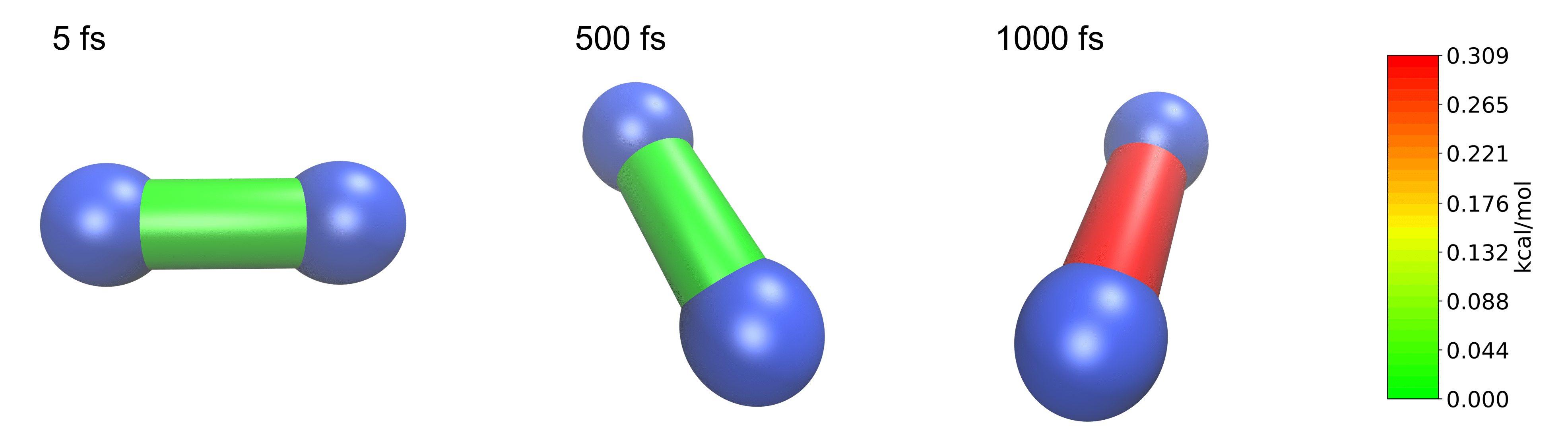
It might be interesting to see the strain energy in bonds during MD simulations since it can show the energy distribution over time. A N2 molecule is simulated at 400 K in the following.
Within ASE using the EMT calculator all necessary data is got by
from ase import Atoms
from ase.calculators.emt import EMT
from ase.optimize import BFGS
from ase.vibrations import Vibrations
n2 = Atoms('N2', [(0, 0, 0), (0, 0, 1.1)],
            calculator=EMT())
BFGS(n2).run(fmax=0.01)

vib = Vibrations(n2)
vib.run()
modes = vib.get_vibrations()


from ase import units
from ase.io.trajectory import Trajectory

from ase.md.langevin import Langevin


T = 400  # Kelvin


atoms = n2.copy()

# Describe the interatomic interactions with the Effective Medium Theory
atoms.calc = EMT()

# We want to run MD with constant energy using the Langevin algorithm
# with a time step of 5 fs, the temperature T and the friction
# coefficient to 0.02 atomic units.
dyn = Langevin(atoms, 5 * units.fs, T * units.kB, 0.002)


def printenergy(a=atoms):  # store a reference to atoms in the definition.
    """Function to print the potential, kinetic and total energy."""
    epot = a.get_potential_energy() / len(a)
    ekin = a.get_kinetic_energy() / len(a)
    print('Energy per atom: Epot = %.3feV  Ekin = %.3feV (T=%3.0fK)  '
        'Etot = %.3feV' % (epot, ekin, ekin / (1.5 * units.kB), epot + ekin))


dyn.attach(printenergy, interval=50)

# We also want to save the positions of all atoms after every 100th time step.
traj = Trajectory('moldyn3.traj', 'w', atoms)
dyn.attach(traj.write, interval=4)

# Now run the dynamics
dyn.run(200)
The Jedi analysis needs to be done for each time step separately. The following generates a Jedi object for each time step comparing it with the optimized state. The visualization scripts for each time step are stored in a different folder named by the parameter “label”. To have a consistent color coding the maximum strain in one bond over the whole simulation is set as the maimum for the color scale with the parameter “man_strain”.
from strainjedi.jedi import Jedi
for i in range(1,51):
    j = Jedi(n2, Trajectory('moldyn3.traj')[i], modes)
    print(Trajectory('moldyn3.traj')[i].calc.get_potential_energy())

    j.run()

    j.vmd_gen(label=str(i), man_strain=0.3087887,modus='all')
Here, three time steps are shown as an example.